Detection is close to solved. Association is the real work. This is a technical note on how a wall-type takeoff pipeline goes from a market-standard ~40-50% to a production ~82% reading accuracy, and how the honest end-to-end number climbs toward that as two named failure modes close. The headline: on production-quality sheets, the pipeline is far above its floor, and the remaining gap to a reliable 90%+ end-to-end is a progression of techniques, not a modeling mystery.
Two problems, still separate
A blueprint shows walls, a legend that defines each type code, a schedule of linear footage per type, and little labels on leader lines pointing at specific segments. A takeoff is done when every wall has the right code and the footage is grouped correctly under it. Detection is a segmentation problem; association is a relational reading problem. We solve them with two independent components, and the whole point of this note is that measuring them honestly requires saying which one you’re testing, on what pages, with which metric.
The honest baselines
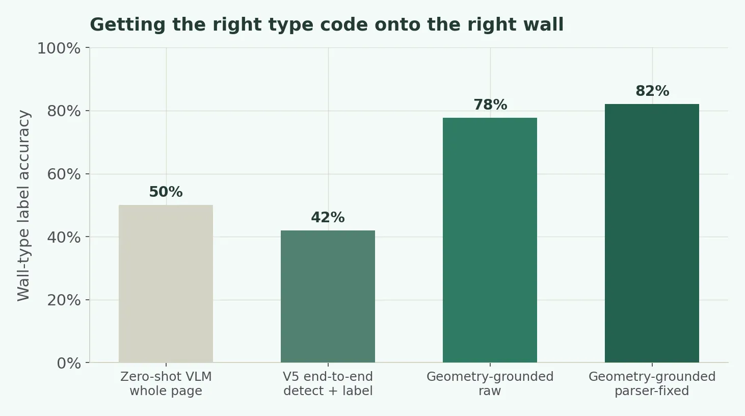
Zero-shot vision-language model (what most demo-day takeoff tools actually do): whole page in, enumerate walls plus codes. On a real page with 95 wall annotations across 21 codes: code-level F1 0.500, precision 1.000, recall 0.333, right about the 7 codes it predicted, silent on 14 of 21, ~7% of linear footage recovered. High precision with low recall is the tell: it plays safe, and a takeoff that finds a third of the types is slower to reconcile than doing it by hand.
A prior end-to-end model (detection plus code in one coupled pass): association F1 0.42 on a validation split. Domain-trained, so better than zero-shot, but coupled, it had to be right about where the wall was AND which code attached, and the errors compounded.
Neither is production. Both are roughly what the market ships.
The move that worked: split the two problems
Detection wants a segmentation prior (long thin regular objects); association wants a reading prior (short strings with almost no geometric structure). One coupled model spends capacity on the wrong thing. So we split them.
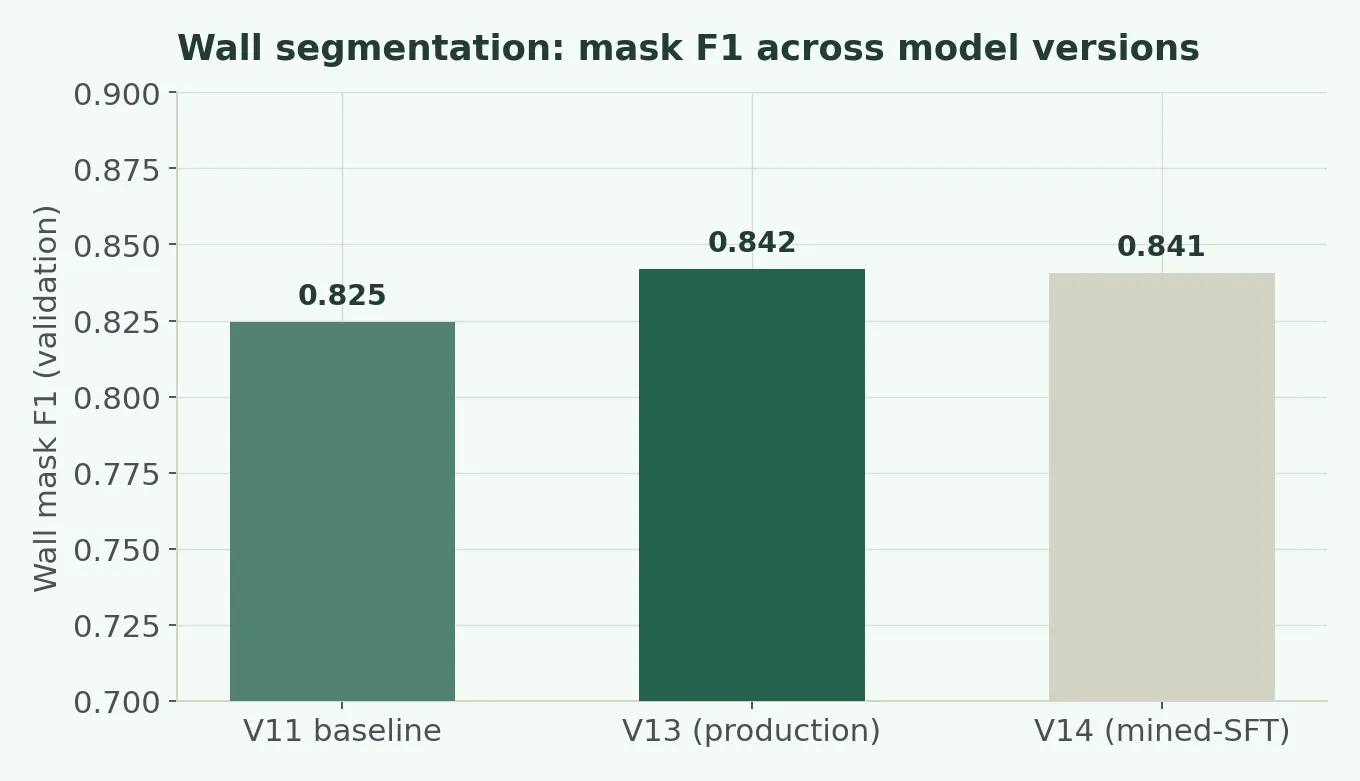
Detection. A multi-head segmentation model with a wall-mask head, a distance-transform centerline head (an auxiliary signal toward a cleaner topological output), and a leader-and-label detection head. The production version reaches mask F1 = 0.842 on a content-crop validation set. A later attempt that added mined training pairs came in flat at 0.841, a useful negative result: at this model capacity we don’t need more data, we need to fix the downstream step.
Association. The winning recipe wasn’t a new model, it was a change in what we show the model. Instead of the whole page, we render a tight crop around a small group of walls (up to 3 per crop, roughly 10% of the page), draw a highly visible axis line down each wall tagged wall-1/2/3, and ask: for each numbered wall, read the type code along its axis line. The model stops finding and starts reading what’s next to something we already marked.
Measuring it honestly
The 82% headline is a reading accuracy on given geometry, the model is handed the wall and reads the code. That is the right metric for the association component, and it is genuinely above 80%. But it is not the end-to-end number, and for a trustworthy claim the two must never be conflated.
So we built a second evaluation deliberately harsher and closer to what a customer experiences:
- Production-faithful inference. The evaluation setup imports the exact production segmentation module and calls the same production inference engine at the same resolution and tiling as the live service, not a reimplementation. Numbers move with production, by construction.
- Larger and end-to-end. 200 pages (140 scored, 60 oversized sheets deferred), 22,122 walls, roughly 2.6x the pages of the component eval and far more walls, scored end-to-end: the model must both find each wall and read its code. A detection miss zeroes the association. This is the pessimistic, production-representative view.
- Strict metric. Segmentation scored with boundary-F1 at 10 pixels over the full page, much stricter on thin walls than pixelwise mask-F1.
Why the end-to-end number is lower than 82%, and why that’s honest. Reading-on-given-geometry (82%) removes the detection-miss penalty entirely. End-to-end folds detection error back in and uses a stricter metric on the full page. They answer different questions. Reporting only the higher one, unlabeled, is exactly the trust failure this note exists to avoid.
The ceiling, established by ablation
The end-to-end mean is a floor, produced with a deliberately weak reader over the full mixed distribution, including a handful of near-empty and pathological sheets. Production runs a stronger reader on production-quality pages. We lifted each source of pessimism, one at a time, to project the ceiling:
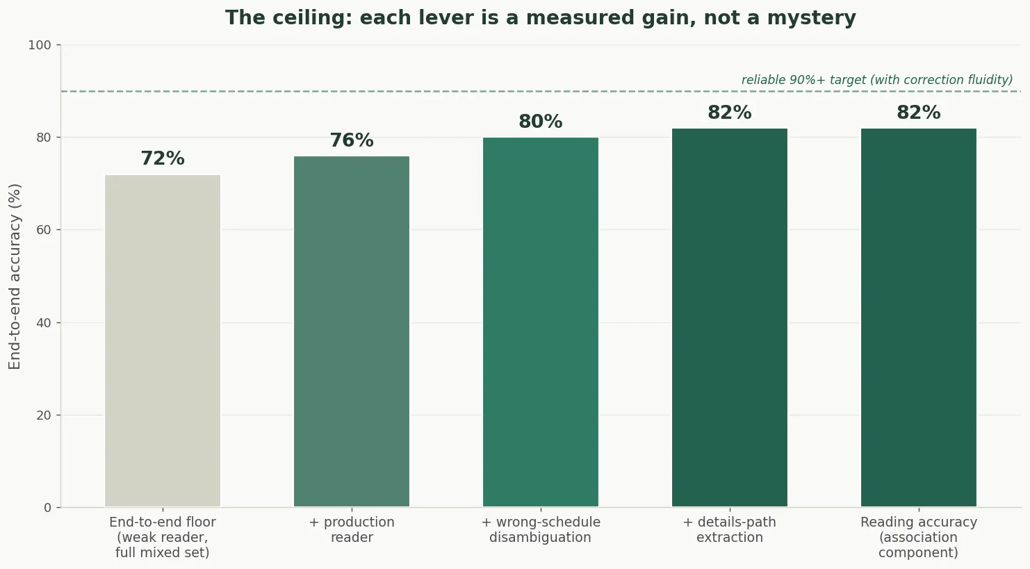
Read this top-to-bottom: the pipeline isn’t stuck at its floor, each lever is a real, measured gain, and the levers are ones we control (reader choice is a config flag; the wrong-schedule and details-path gaps are named failure modes below). On clean production-quality sheets the detector is already at roughly 0.92 boundary-F1 / 0.842 mask-F1, walls are, for practical purposes, found. The end-to-end ceiling with the production reader lands around 0.72 and climbs toward the ~82% reading accuracy as the two remaining gaps close.
What caps the end-to-end number
The errors cluster, none are wild hallucinations, every one is a specific, addressable failure mode:
- Wrong-schedule selection is the single biggest lever. On multi-schedule sheets the reader sometimes locks onto a sibling table (door, fire, or finish) instead of the wall-type legend, and when it does, the segmentation is often perfect (boundary-F1 0.92-0.98) while the label is simply from the wrong vocabulary. Roughly a quarter of pages show this. A stronger reader already cuts it sharply (wrong-schedule pages dropped from 11 to 4 of 50 when we moved from a weaker reader to the production reader). Explicit legend-and-schedule disambiguation is the highest-value next fix. This alone moves the end-to-end mean most.
- The details path, roughly 40% of codes aren’t in the schedule table at all. They live in plan details: exploded partition views with the fire rating in text. We read schedules well and details poorly. A structured detail-extraction model is now in production, and the association pipeline is being extended to pull from details as well as schedules. When it lands, the ceiling moves again.
- Variant-code depth (e.g.
P1.3vsP1,ASW6.2vsASW6), a granularity question about how deep a code the takeoff needs, resolved by the scoring convention, not the model.
Close (1) and (2) with the production reader on production sheets, and the honest end-to-end number tracks the component reading accuracy into the 80s, the same ~82% the association step already achieves in isolation, now earned end-to-end.
What this unlocks
Association is now accurate enough that a takeoff is faster to audit than to do, the crossover where the human’s job shifts from redoing the work to correcting the model, and total time drops from days to hours. Detection and association improve on independent loops: tighten the mask, association gets cleaner crops; improve the reader, no detection retrain. Two teams, two loops, no coupling.
The number the user feels is higher
Everything above is pure model accuracy on a static benchmark. What a customer experiences in the product is a different, higher number, and it’s worth being precise about where the extra points come from, because none of them require touching model weights.
Perceived accuracy is model accuracy multiplied by the fluidity of correction. A takeoff isn’t a one-shot prediction the user accepts or rejects; it’s a high-bandwidth surface they steer. When the model labels 72% of a sheet correctly and the remaining walls are one click to fix, the wall is already detected, the code list is already known from the legend, the correction is a dropdown, not a redraw, the effective accuracy the user walks away with is far above the raw model number. The design goal for the UI is to make every residual error cheap to catch and cheap to fix: grouped by code, footage totaled live, low-confidence labels flagged for review first. Model accuracy sets the floor; correction fluidity sets what the user feels, and together they land the perceived accuracy in the 90s.
And the fastest iterations aren’t retrains, they’re association prompt techniques. Updating segmentation weights is a days-long loop (data, train, export, validate, redeploy the inference engine). The association reader, by contrast, is steered by how we prompt it, and those levers ship in hours. Three that are live in production today, all pure prompt-and-render-and-config, no weights:
- Smart clustering. Walls are grouped into small spatial clusters and each cluster is one crop, one call. Natural groups up to around 20 walls are kept whole; only genuinely dense groups are split into tight grid cells (around 12) so numbered markers stay legible. This trades call count against crop legibility with a single constant, retuned in minutes, not a training run.
- Numbered-index-circle indexing. Each wall in a crop is identified solely by a numbered circle drawn on it, so the reader references walls by index rather than by re-describing geometry. It decouples “which wall” from “what code” and makes the reply trivially parseable.
- Legend vs. self-discovery, with graceful fallback. A first pass reads the sheet’s own wall-type legend and constrains the reader to that vocabulary; if too many proposed labels miss the legend (a wrong or partial legend, a real and common failure), the page automatically re-runs in self-discovery mode, free-reading codes off the drawing. On a dense-page evaluation this fallback lifted assembly-core accuracy from 60.9% to 75.7%, a large gain shipped as a prompt-flow change, with zero retraining.
That’s the practical thesis of this whole effort: once detection is solved, the accuracy the user feels is bought far more cheaply on the prompt-and-product side than in the weights. Retraining moves the segmentation floor slowly; prompt techniques move the association number fast; and a fluid correction surface converts an honest 72-82% model into a 90%+ experience.
Where this goes next
The immediate mile is the details path (item 2 above). The next is per-trade generalization: this was architectural walls (partitions, fire ratings, assemblies); concrete, structural, and curtain walls each carry a different codebook. The geometry-grounded recipe transfers, but each trade needs its own validation set and audit pass.
The story, still: don’t ask one system to do two jobs. Detection is a segmentation problem, association is a reading problem, and once you measure each on its own honest terms, you can say exactly how far you are from 80%+, which lever gets you there, and why the number the user feels is already higher than the number on the benchmark.